If you use a Google Form to collect data email addresses, then you may want to use the Forms data-validation tool to check that the entered addresses are at least in the right "shape" to be email addresses.

Transferring ownership of a Google Sheets file

And you can share these files with any other Google account.
But there are some limits about which of these files you can make someone else the owner of:
- Google Apps Customers: can't transfer ownership of any file to someone outside your domain.
- Only Google Apps customers in Premier, Government, and Education domains can transfer ownership of a synced or uploaded file (like a PDF or image file) - and of course this is only to someone in your own domain.
- Consumer (ie non corporate / organisation wide) Google Drive users: can't transfer ownership of a synced or uploaded file (ie a file that started its life on your own personal machine) - but you can transfer ownership of files that you created inside Apps itself.
Apart from these, you can transfer ownership of Google documents and folders to anyone else, as long as they have an email address which either is already linked to a Google account, or they are willing to set up a Google account for
How to make someone else the owner of a spreadsheet file
Go to Google Drive
Tick the check-box beside (currently on the left side of) the file or folder you want to transfer
From the More menu, choose"Share..." - or just click the Share icon.
Give access to the person you want to give the file ownership to (unless they already have it) - and if they aren't an existing Google user, wait for then to accept the invitation and thus show up on the list of people with access.
In the Sharing screen, click the drop-down menu on the right hand side of the new owner's name, and choose "Is owner."
Click Save changes.

Job Done! The person now owns the file - and you don't own it any more.
What happens after your transfer ownership in this way
The new owner will get an email telling them that they have been made the owner of the file.You will still be an editor on the file. But because you are no longer the owner, you won't be able to:
- Remove existing collaborators
- Share the file with other people
- Change the visibility options (ie who else can see the spreadsheet)
- Give collaborators permission to change other people's access privileges
- Delete the file. (You can remove it from the list of files that are shared with you, but it will still be in the new owner's Google Drive)
Acknowledgements
This post expands on the official Google support post at https://support.google.com/drive/answer/2494892?hl=enHow to name a column (or row) in a Google Spreadsheet

The same approach can be used for rows - you simply need to use the word "row" instead of "column" in the following directions.
Give someone else access to a Google Spreadsheet that you have created

For example, recently my choir's recruitment co-ordinator was on holiday during a week when we knew that some people would contact us to ask about membership. By giving me edit-access to the audition-scheduling spreadsheet, I could look after these messages for her, and she had immediate access to the up-to-date information when she came home.
Giving everyone in the whole world (well at least everyone with a Google account) access is very easy: you just change the first, generic, option in the access control lists.
But giving access to specific individual people is a little more desirable and only a tiny bit harder to set up.
Adding values in one column, based on another one, using the SUMIF function
This post explains how to calculate the total of the values in one row or column, based on the corresponding values in another related row or column, using the SUMIF function in Google Sheets.

New tool for using Google Sheets on your smartphone or tablet
Google have announced new apps for several components of their Drive software, including Google Sheets.
They say this makes it possible to create content on the go - but even with a very new smartphone, I'm finding it hard to imagine making a spreadsheet of any size. It just feels weird to have the formula-bar at the bottom of the screen.
And I've had some "interesting" experiences browsing a spreadsheet created in the desktop version which records the responses to a questionnaire created in Google Forms, which has a lot of long text-fields: it's easy to hide a column by accident, and without a shift-key I'm not sure how to make visible again.
But overall I like the idea, especially the way that I can effectively use Sheets as a calculator app which lets me see and easily change my on-the-go calculations. And I can imagine that it could be a handy way to build some highly targeted "mini-apps" to do particular calculations in a spreadsheet, without the overhead of installing a separate app.
 |
| Screenshot of the new Google Sheets app for Android |
They say this makes it possible to create content on the go - but even with a very new smartphone, I'm finding it hard to imagine making a spreadsheet of any size. It just feels weird to have the formula-bar at the bottom of the screen.
And I've had some "interesting" experiences browsing a spreadsheet created in the desktop version which records the responses to a questionnaire created in Google Forms, which has a lot of long text-fields: it's easy to hide a column by accident, and without a shift-key I'm not sure how to make visible again.
But overall I like the idea, especially the way that I can effectively use Sheets as a calculator app which lets me see and easily change my on-the-go calculations. And I can imagine that it could be a handy way to build some highly targeted "mini-apps" to do particular calculations in a spreadsheet, without the overhead of installing a separate app.
The Sheets app vs the Drive app
This comment from Google sums up the difference - bolding mine:use the Drive app to view and organize all of your documents, spreadsheets, presentations, photos and more.And by implication, use the Sheets, (and Docs, and when it arrives Slides) app to change (ie edit) your spreadsheets et al.
How to combine a cell value and a text-string
Sometimes you may want to write a formula which combines the value(s) from some cells with some other text, and puts the result into the one cell.
For example, I have a spreadsheet which generates the HTML code statements for drawing a table, based on the values which I put into a table-area on the spreadsheet. And I need to combine the values from the table area with other HTML commands like "" and ""

The way to do this in Google Spreadsheets is to use a string concatenation operator (&) or a string-concatenation function ( CONCAT( , ) or CONCATENATE(...) )
For example, I label the value from C5 with the text "Score type:", and so in the results column which I use to make the table-cell code for it, the formula is:
Or a less verbose way to achieve the same thing is:
The CONCATENATE() can be used to join any number of text strings together, so another way to write the statement is
In general, it's best to use the option which makes the formula the most readable, or easiest to diagnose if something goes wrong.
So often I will use the CONCAT() function in each one of a set of helper columns, and then use one CONCATENATE() function at the end to join them all together, because this is easier to debug than trying to do a lot of string operations all in the one cell.
For example:

For example, I have a spreadsheet which generates the HTML code statements for drawing a table, based on the values which I put into a table-area on the spreadsheet. And I need to combine the values from the table area with other HTML commands like "" and ""
The way to do this in Google Spreadsheets is to use a string concatenation operator (&) or a string-concatenation function ( CONCAT( , ) or CONCATENATE(...) )
For example, I label the value from C5 with the text "Score type:", and so in the results column which I use to make the table-cell code for it, the formula is:
=CONCAT("<td>Score type: ", CONCAT(C5, "</td>"))
Or a less verbose way to achieve the same thing is:
="<td>Score type: " & C5 & "</td>"
What's the difference between "&" CONCAT and CONCATENATE?
The CONCAT() function and the "&" operator do the same thing, so whether you use one or the other is is about which one looks nicer to you.The CONCATENATE() can be used to join any number of text strings together, so another way to write the statement is
=CONCAT("<td>Score type: ", C5, "</td>"))
In general, it's best to use the option which makes the formula the most readable, or easiest to diagnose if something goes wrong.
So often I will use the CONCAT() function in each one of a set of helper columns, and then use one CONCATENATE() function at the end to join them all together, because this is easier to debug than trying to do a lot of string operations all in the one cell.
For example:
Was this helpful? You might also like:
How to refer to a range in another sheet
If you use multiple worksheets in a spreadsheet, then you can refer to an individual cell in a worksheet - including one that you are not currently working in - like this:
And you can even combine values from different sheets by putting different sheet-name references into a formula like this;
This makes some people think that they should refer to a range of cells in a different worksheet (eg B1:b16) like this:
However using this formula shows #ERROR! as a result, with a not-very-helpful error message of "Formula Parse Error".

The correct way to refer to a range of cells in a separate worksheet is to use the sheet-name only once, like this:
The reason for this is that within the one function call (eg SUM(...) or AVERAGE(...) ) all the cells must come from the same worksheet. It does not make any sense to say:
But it does make sense to combine function calls like this:

For functions like AVERAGE, where the number of items in the underlying range is used in the calculation, it does not work, eg
=Sheet2!B1
(A formula like this returns the value in Worksheet Sheet2, Cell B1.)
And you can even combine values from different sheets by putting different sheet-name references into a formula like this;
=Sheet2!B1 + Sheet3!B1
(A formula like this returns the value in Worksheet Sheet2, Cell B1 plus the value in Worksheet Sheet3, Cell B1)
This makes some people think that they should refer to a range of cells in a different worksheet (eg B1:b16) like this:
=SUM(Sheet2!B1:Sheet2!B16)
However using this formula shows #ERROR! as a result, with a not-very-helpful error message of "Formula Parse Error".
The correct way to refer to a range of cells in a separate worksheet is to use the sheet-name only once, like this:
=SUM(Sheet2!B1:B16)
(A formula like this returns the sum of values in cells B1:B16 in Sheet2.)
The reason for this is that within the one function call (eg SUM(...) or AVERAGE(...) ) all the cells must come from the same worksheet. It does not make any sense to say:
=SUM(Sheet2!B1:Sheet3!B16)because it's not defined what is in-between Sheet2 and Sheet3.
But it does make sense to combine function calls like this:
=SUM(Sheet2!B1:B16) + =SUM(Sheet3!B1:B37)
(A formula like this returns the sum of values in cells B1:B16 in Sheet2, plus values in cells B1:B37 in Sheet3)
Extra for Experts
Of course this only works if they type of function that you are using is distributitive, ie you can do one part and the other part, and then you put them both together using the same functon, eg= MIN ( MIN(Sheet2!B1:B16), MIN(Sheet3!B1:B22))
(A formula like this returns the smallest value in cells B1:B16 in Sheett and cells B1:B37 in Sheet3)
For functions like AVERAGE, where the number of items in the underlying range is used in the calculation, it does not work, eg
= AVERAGE ( AVERAGE(Sheet2!B1:B16), AVERAGE(Sheet3!B1:B22))will give a result but it will generally not be the arithmetic mean of the value in cells B1:B16 in Sheett and cells B1:B37 in Sheet3 because the values from Sheet2 will get too great a weighting in the calculation.
Was this helpful? You might also like:
How to find the difference between two time values
Calculating the difference between two times (or date-times) in Google Spreadsheets is just as simple as calculating the difference between two dates, provided the time values are formatted as Times.
You simply do a "minus" between the later time and the earlier one.
At its simplest, you just do a minus calculation, like this:
The result that is shows is the time differences, expressed as the number of days between the two values.
You may want to do further calculations, or apply Duration formatting, to make this number more user-friendly.

If you need to cover these cases, then check back again soon, so see posts explaining how to handle these situations.
Display formats and date / time differences
You simply do a "minus" between the later time and the earlier one.
At its simplest, you just do a minus calculation, like this:
C5 = C4 - C3
The result that is shows is the time differences, expressed as the number of days between the two values.
You may want to do further calculations, or apply Duration formatting, to make this number more user-friendly.
Troubleshooting
If it looks like your time difference calculation is not working correctly, then then are are few things to check.- Are your time values (ie not just the result) formatted as Times?
Check this under menu: Format > Number > Time.
NB It is not the same as the Font of "Times", which is totally different
- Do you know that what is shown is the number of days, and this may be a fraction or decimal value.
Possibly it is not formatted the way you want it to be.
Check the formatting under Format > Number, and remember that 15 minutes = 0.25 of an hour, or 0.010416667 of a day.
Extra for experts
A simple minus calculation only works correctly if:- Both times are in the same time-zone
- If the later time is on a different day, then the values that you are calculating on must both have a "date" part as well as a "time" part.
If you need to cover these cases, then check back again soon, so see posts explaining how to handle these situations.
Was this helpful? You may also need to read
Calculating the difference between two datesDisplay formats and date / time differences
Why date calculations sometimes need to have +1 added to them: whole vs partial days
When people prepare a list of start and end dates, they generally assume that the start and end date are both included.
 .
.
For example, in my summer school management spreadsheet, start-date of 3-June actually means "9am on 3 June", and end-date of 6-June actually means "5pm on 6 June" - even though I haven't explicitly named the times.
But spreadsheets do not work like this: if they see a date value with out a time, then they assume that it means 12-midnight at the beginning of that day.
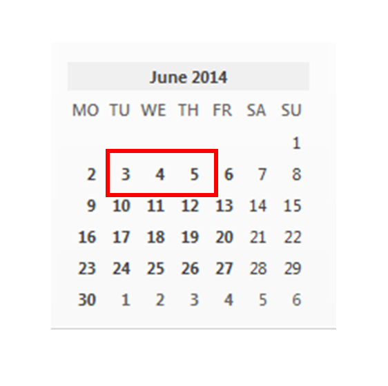
For example, Google Spreadsheets understands
Therefore when a spreadsheet is told to calculate the difference between these two date values, if works out the number of whole days between the two values.
In the example shown, this is three days
However most people would expect the calculation to return four days, ie to include both the start-date and the end date, and the result to equal four days
There are two ways to fix this:
It becomes
This is the simplest approach, and is best when you do not need to consider times in your calculations.
Instead you alter the values that the calculation is based on, adding a time-part to them.
This works - but the result of a difference calculation is the actual number of days between the two values, expressed as a whole number, ie with a decimal point.
eg 9am on 13 June to 5 pm on 19 June returns 4.333333333
This may be ok in some cases, eg if you just want to know if the duration is greater than a certain value.

But if you actually want to show the number of days, even if they are not complete days, then you may need to use a function like ROUNDUP(value, places) as well as the subtraction formula.
To do this, the function becomes:
The ", 0" in the formula says to round the value up to the nearest integer, ie number with zero decimal places.

Display formats and date / time differences
For example, in my summer school management spreadsheet, start-date of 3-June actually means "9am on 3 June", and end-date of 6-June actually means "5pm on 6 June" - even though I haven't explicitly named the times.
But spreadsheets do not work like this: if they see a date value with out a time, then they assume that it means 12-midnight at the beginning of that day.
For example, Google Spreadsheets understands
- "start-date of 3-June" as "3-June, 00:00:00"
- "end-date of 6-June" as "6-June, 00:00:00".
Therefore when a spreadsheet is told to calculate the difference between these two date values, if works out the number of whole days between the two values.
In the example shown, this is three days
However most people would expect the calculation to return four days, ie to include both the start-date and the end date, and the result to equal four days
There are two ways to fix this:
Option 1: Add one to the results
Under this option, you need to change the formulaIt becomes
=D4-C4+1
This is the simplest approach, and is best when you do not need to consider times in your calculations.
Option 2: Add times to the date values
Under this option, you do not need to change the formula.Instead you alter the values that the calculation is based on, adding a time-part to them.
This works - but the result of a difference calculation is the actual number of days between the two values, expressed as a whole number, ie with a decimal point.
eg 9am on 13 June to 5 pm on 19 June returns 4.333333333
This may be ok in some cases, eg if you just want to know if the duration is greater than a certain value.
But if you actually want to show the number of days, even if they are not complete days, then you may need to use a function like ROUNDUP(value, places) as well as the subtraction formula.
To do this, the function becomes:
=RoundUp(D4-C4, 0)
The ", 0" in the formula says to round the value up to the nearest integer, ie number with zero decimal places.
Was this helpful? You may also need to read
Calculating the difference between two timesDisplay formats and date / time differences
How to show the difference between two dates
Finding out how long between two dates in a Google Spreadsheet is very simple: you just subtract the later one from the earlier one, like this:

Looking in more detail at what happens on the spreadsheet in this formula, you just need to
Google Sheets uses colour-coding in the cells and dotted lines to help you see exactly what cells the formula is pointing to.

Looking in more detail at what happens on the spreadsheet in this formula, you just need to
- Type an equals sign ("=") - this tells the spreadsheet that you are going to put a formula into that cell
- Type (or point to) the later value
- Type a minus sign ("-")
- Type (or point to) the earlier value
- Press Enter
Google Sheets uses colour-coding in the cells and dotted lines to help you see exactly what cells the formula is pointing to.
Was this helpful? You may also need to read:
- Date-calculations and Plus-One: whole vs partial days
- Calculating the difference between two times
- Google Sheets date-format effects on calculation results
Understanding Google Sheets, Spreadsheets and Worksheets
There's a great discussion which many people have had, about the difference between email and Gmail.
The short answer is "Gmail is a type of email system". But to really make sense of this, you need to "get" the difference between email messages, the concept of email message handling, and being able to use different front-end applications to look at the same email message. If someone doesn't have this idea, then their immediate response to "Gmail is a type of email" is "Ok then, so what is fmail?"
I have a nasty feeling that Google's choice to name all their office-applications by such generic names (Sheets, Docs, Slides) is likely to lead to the same confusion in more areas.

This post is an attempt to simply explain the basic concepts of spreadsheets, Google Sheets, and worksheets within sheets.
It is different from a word-processor (eg Microsoft Word or Google Docs), because it has tools that make doing mathematical / arithmetic calculations easy.
It is different from a database (eg Microsoft Access, MySQL) because it doesn't force you to put data into every single row and column that it has, and it has very easy-to-use tools to make attractive displays.
It is different from a Slides file, because it does not use slides to display the data in it.
There are various ways to organize spreadsheets, but fundamentally each one is a file that is divided up into a grid made up of rows and columns,

The intersection of each row and column is a cell.
Each cell is named according to the row and column that make it up. Normally the column name goes first, and the

In each cell you can put either text (ie words), numbers, or formulas ie calculations that take the values from other cells, combine them in some way and then display the results.
For example, the picture below shows the beginnings of a spreadsheet that contains the timetable for a summer school. I've done it in a spreadsheet, rather than an Document file, because I want to use some calculation and summary functions, as well as making it look professional.

Sometimes is it short for "spreadsheet file". This has a file which has the structure described above and which can be used by a spreadsheet program.
Sometimes it means "spreadsheet proram". This is a piece of software (aka an application) which is used to create and work with spreadsheet files. Spreadsheet programs may be on-line (like Google Sheets), or run on individual computers (like Excel or Lotus 1-2-3).
Because of this double-meaning, you can write some very strange sentences in English, eg
Google now distinguish between
But that size can be quite overwhelming: it can be hard to find things in spreadsheets that other people made, and it can be difficult to make different "views" which all look good, because each column has to be the same width through the whole sheet.
So the concept of Tabs was introduced. Basically the are extra layers of the the spreadsheet, stored in the same file.
In almost all spreadsheet programs (including Google Sheets), you see the tabs at the bottom left hand corner

In both Microsoft Excel and Google Sheets (the program), these tabs are called Worksheets.
But they have default names "Sheet1", "Sheet2", etc so sometimes people just call them sheets, and talk about "Sheet2 in the sheet" - and this can be very confusing if you're not sure of the difference.
 If there are several worksheets in a sheet, then the name of each cell becomes:
You can add a new worksheet to your Google Sheets file using the plus sign on the very left hand side of the bottom tab bar

The short answer is "Gmail is a type of email system". But to really make sense of this, you need to "get" the difference between email messages, the concept of email message handling, and being able to use different front-end applications to look at the same email message. If someone doesn't have this idea, then their immediate response to "Gmail is a type of email" is "Ok then, so what is fmail?"
I have a nasty feeling that Google's choice to name all their office-applications by such generic names (Sheets, Docs, Slides) is likely to lead to the same confusion in more areas.
This post is an attempt to simply explain the basic concepts of spreadsheets, Google Sheets, and worksheets within sheets.
What is a spreadsheet?
A spreadsheet is a row-and-column based tool for working with data on a computer.It is different from a word-processor (eg Microsoft Word or Google Docs), because it has tools that make doing mathematical / arithmetic calculations easy.
It is different from a database (eg Microsoft Access, MySQL) because it doesn't force you to put data into every single row and column that it has, and it has very easy-to-use tools to make attractive displays.
It is different from a Slides file, because it does not use slides to display the data in it.
There are various ways to organize spreadsheets, but fundamentally each one is a file that is divided up into a grid made up of rows and columns,
The intersection of each row and column is a cell.
Each cell is named according to the row and column that make it up. Normally the column name goes first, and the
In each cell you can put either text (ie words), numbers, or formulas ie calculations that take the values from other cells, combine them in some way and then display the results.
For example, the picture below shows the beginnings of a spreadsheet that contains the timetable for a summer school. I've done it in a spreadsheet, rather than an Document file, because I want to use some calculation and summary functions, as well as making it look professional.
Spreadsheet files vs Speadsheet programs
The word "spreadsheet" is actually an abbreviation.Sometimes is it short for "spreadsheet file". This has a file which has the structure described above and which can be used by a spreadsheet program.
Sometimes it means "spreadsheet proram". This is a piece of software (aka an application) which is used to create and work with spreadsheet files. Spreadsheet programs may be on-line (like Google Sheets), or run on individual computers (like Excel or Lotus 1-2-3).
Because of this double-meaning, you can write some very strange sentences in English, eg
"I will use my spreadsheet to make a spreadsheet to calculate the spread of sheets through the hotel."meaning
"I will use my spreadsheet-program to make a spreadsheet-file to calculate the distribution of bed linen through the hotel."
Google now distinguish between
- Google Drive, ie the software that you use to manage files (or any type), and
- Google Docs ie the Document, Spreadsheet, Presentation, Form or Drawing objects that you can create inside Drive.
Spreadsheets vs Sheets / Worksheets
To start with, a spreadsheet is like a big blank canvas, waiting for you to put numbers and formulae into it.But that size can be quite overwhelming: it can be hard to find things in spreadsheets that other people made, and it can be difficult to make different "views" which all look good, because each column has to be the same width through the whole sheet.
So the concept of Tabs was introduced. Basically the are extra layers of the the spreadsheet, stored in the same file.
In almost all spreadsheet programs (including Google Sheets), you see the tabs at the bottom left hand corner
In both Microsoft Excel and Google Sheets (the program), these tabs are called Worksheets.
But they have default names "Sheet1", "Sheet2", etc so sometimes people just call them sheets, and talk about "Sheet2 in the sheet" - and this can be very confusing if you're not sure of the difference.
- The sheet name
- An exclamation mark
- The row-and-column reference.
In the picture above, these are all separate cells:
- Timetable!B5 - which is on the Timetable tab / sheet
- Registrations!B5 - which is on the Registrations tab / sheet
- Sheet6!B5 - which is on a sheet called Sheet6 (you cannot see this in the picture)
You can add a new worksheet to your Google Sheets file using the plus sign on the very left hand side of the bottom tab bar
How to combine a range of values into one cell, with a character in between them
If you have a list of items in a spreadsheet, set up like a table, then you can use the join function to combine the values and display them all together in a horizontal list, with some characters (eg a comma and a space) in between tehm..
For example, in my summer-school management spreadsheet I have a list of teachers in column C, currently in rows 1 (heading) to five.
Teachers
-----------
Fiona
Patrick
Sean
Lynne
To put the teacher-names into the one cell, nicely formatted with a comma and a space between each one, I could use the JOIN() function, like this:
But there are two problems:
A better option it to also use the FILTER() function, to remove values that you dont't want in this case, blanks which are represented by "".
So the formula becomes:
Using this, my list becomes "Fiona, Patrick, Sean, Lynne", and I can add up to 9998 names in the Teachers column and it still works.

For example, in my summer-school management spreadsheet I have a list of teachers in column C, currently in rows 1 (heading) to five.
Teachers
-----------
Fiona
Patrick
Sean
Lynne
To put the teacher-names into the one cell, nicely formatted with a comma and a space between each one, I could use the JOIN() function, like this:
= JOIN( ", " ; C2:C5 )
But there are two problems:
- The result is "Fiona, Patrick, Sean, Lynne, " - there is an extra "comma space" at the end
- If the number of teachers changes, the I have to adjust the formula
A better option it to also use the FILTER() function, to remove values that you dont't want in this case, blanks which are represented by "".
So the formula becomes:
= JOIN( ", " ; FILTER(C2:C9999; NOT(C2:C999 = "") ))This says to join all the values in cells C2 through to C9999 together, to put a comma and space between each one, but to leave out any that are blank,
Using this, my list becomes "Fiona, Patrick, Sean, Lynne", and I can add up to 9998 names in the Teachers column and it still works.
Extra for Experts
If I had used named ranges, and so didn't have a heading at the top of the column, then the formula could become even more flexible, with no limit to the number of rows included, like this:= JOIN( ", " ; FILTER(C:C; NOT(C:C = "") ))
or
= JOIN( ", " ; FILTER(Teachers; NOT(Teachers = "") ))
Where to get help with Google Sheets
Google's Getting started guide:
https://support.google.com/drive/topic/20322Google's own help pages for sheets
https://support.google.com/drive/topic/20322?hl=en-GB&ref_topic=2811806The Google Docs product forum:
https://productforums.google.com/forum/#!forum/docsThis has questions and answers about all types of Google Drive/ Google Docs files.
StackExchange Webapps GoogleSheets category
http://webapps.stackexchange.com/questions/tagged/google-spreadsheets
Excel Help Forum
http://www.excelforum.com/for-other-platforms-mac-google-docs-mobile-os-etc/This privately-run forum has a thread for other spreadsheet tools, including Google Docs.
What other help sites have you found?
Leave a comment below, and I'll add them to the list.
Subscribe to:
Posts (Atom)