Why date calculations sometimes need to have +1 added to them: whole vs partial days

When people prepare a list of start and end dates, they generally assume that the start and end date are both included.

.
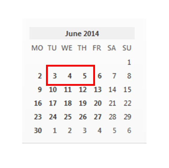
For example, in my summer school management spreadsheet, start-date of 3-June actually means "9am on 3 June", and end-date of 6-June actually means "5pm on 6 June" - even though I haven't explicitly named the times.

But spreadsheets do not work like this:   if they see a date value with out a time, then they assume that it means 12-midnight at the beginning of that day.


For example, Google Spreadsheets understands

• "start-date of 3-June" as "3-June, 00:00:00"
• "end-date of 6-June" as "6-June, 00:00:00".

Therefore when a spreadsheet is told to calculate the difference between these two date values, if works out the number of whole days between the two values.

In the example shown, this is three days

However most people would expect the calculation to return four days, ie to include both the start-date and the end date, and the result to equal four days

There are two ways to fix this:

Option 1:  Add one to the results

Under this option, you need to change the formula

It becomes

=D4-C4+1

This is the simplest approach, and is best when you do not need to consider times in your calculations.

Option 2:  Add times to the date values

Under this option, you do not need to change the formula.

Instead you alter the values that the calculation is based on, adding a time-part to them.

This works - but the result of a difference calculation is the actual number of days between the two values, expressed as a whole number, ie with a decimal point.

eg    9am on 13 June to 5 pm on 19 June returns 4.333333333

This may be ok in some cases, eg if you just want to know if the duration is greater than a certain value.

But if you actually want to show the number of days, even if they are not complete days, then you may need to use a function like ROUNDUP(value, places)  as well as the subtraction formula.

To do this, the function becomes:

=RoundUp(D4-C4, 0)

The ", 0" in the formula says to round the value up to the nearest integer, ie number with zero decimal places.

Was this helpful? You may also need to read

Calculating the difference between two times
Display formats and date / time differences